Let’s build a simple journey planner using SQL (part 1 of definitely more than 1)

Published: 1 Jun 2023
Updated: 1 Jul 2023
Written by: Chun Fei Lung

When all you have is a relational database, everything looks like a table. And you know what? It works! Sort of.

Oh, would you look at the timetable?

It already says so in the title, but I’ll repeat it here just in case you didn’t notice the huge text above the article: today we’re going to build a simple journey planner in SQL using everyone’s ~~favourite~~ barely tolerated relational database, MySQL (side note: Actually, I’m lying. It’s MariaDB.). Although this is not a particularly good idea, it is an idea and therefore I’m going to run with it.

I could create a small toy network to demonstrate how this works, but to keep things a bit more interesting I’m going to do this with real public transport data.

Let me show you to your tables

We’ll make use of a public GTFS static feed for all public transport in the Netherlands, which is published under a CC0 license. For now, we’ll only consider trains, because reasons.

Timetables

GTFS feeds include a lot of useful information (side note: A complete overview can be found on the Google Transit website.), but we only need to load a subset of this data into the database. I’ll give a brief description of each table that I imported, along with a few example rows that should give you an idea of what it contains.

agency

Public transport services are operated under a brand, i.e. an agency. Most travellers will think of a brand as the company that offers services. In practice a company may operate under multiple brands, and some brands are used by multiple companies.

id	name
1	Eurobahn
2	Valleilijn
8	R-net
9	NS
11	Breng
12	NS International
15	Arriva
17	Blauwnet
22	Eu Sleeper
26	VIAS

route

Routes are what most people would call lines. Routes are associated with a transportation type (e.g. trams, metros, trains, and buses). From a traveller’s perspective lines are generally identified by a number, a letter or a name. Not to be confused with the exact path that a vehicle travels along, which is called a “shape” in GTFS parlance.

id	agency_id	short_name	long_name	type
22	9	Sprinter	Tilburg Universiteit <-> Weert SPR6400	2
23	12	Eurostar	Amsterdam Centraal <-> London St. Pancras Int. EST9100	2
24	12	Intercity	Amsterdam Centraal <-> Berlin Ostbahnhof IC140	2
71	9	Intercity	Schiphol Airport <-> Nijmegen IC3100	2

trip

Each route is served by trains that make trips (often in one direction or the other) throughout the day. The headsign informs travellers of the final destination of the train.

id	route_id	headsign
3847	24	Amsterdam Centraal
3848	24	Berlin Ostbahnhof
1807	71	Schiphol Airport
1808	71	Nijmegen
5408	71	Schiphol Airport
5409	71	Nijmegen

stop

Vehicles stop at stops. Somewhat confusingly, a stop can be anything from a bus stop pole to (part of) a platform to an entire station. Technically it can also be other things, but we’re just going to ignore that for now.

id	name	latitude	longitude	platform
35025	Nijmegen	51.843352716672	5.8527283567859	1
35026	Nijmegen	51.8440139658	5.85304677486	1a
35027	Nijmegen	51.842415589576	5.8522424471402	1b
35028	Nijmegen	51.843418123199	5.8525284242761	3
35030	Nijmegen	51.8440338507	5.85280001163	3a
35031	Nijmegen	51.842471977321	5.8520218494775	3b
35032	Nijmegen	51.843382598179	5.8523051845771	4
35033	Nijmegen	51.8440537357	5.85269272327	4a
35034	Nijmegen	51.842489994433	5.851883317404	4b
35029	Nijmegen	51.842214820937	5.8522482783764	35
35035	Nijmegen	51.843845719325	5.8534115553016
35036	Nijmegen	51.842718896418	5.852064148637
47601	Nijmegen	51.8432285026	5.85303068161
35045	Nijmegen Heyendaal	51.8268250995	5.86774528027	1
35046	Nijmegen Heyendaal	51.826879804	5.86788743734	2
35047	Nijmegen Heyendaal	51.8266261734	5.86765944958
35048	Nijmegen Heyendaal	51.8266261734	5.86765944958

The table above shows the records for two train stations, “Nijmegen” and “Nijmegen Heyendaal”. The first train station has four platforms (1, 3, 4, and 35), some of which are subdivided into an “a” and “b” section. The second, local station only has two platforms.

stop_time

Stop times are the main component of a timetable. The data in this table can be used to deduce which lines serve a particular stop, when vehicles arrive and depart at stops, how many stops a line has (and skips), and what the distance between each stop is.

id	trip_id	stop_id	stop_sequence	arrival_time	departure_time	shape_dist_traveled
25541	1807	35028	1	2023-06-01 15:28:00	2023-06-01 15:28:00	1
4395	1807	33353	5	2023-06-01 15:40:00	2023-06-01 15:45:00	18394
4396	1807	34041	8	2023-06-01 15:55:00	2023-06-01 15:55:00	34741
39696	1807	34705	9	2023-06-01 16:01:00	2023-06-01 16:01:00	41835
54327	1807	35518	14	2023-06-01 16:19:00	2023-06-01 16:26:00	75049
54328	1807	33511	20	2023-06-01 16:42:00	2023-06-01 16:44:00	104460
39697	1807	33569	22	2023-06-01 16:49:00	2023-06-01 16:51:00	110602
4397	1807	35346	23	2023-06-01 16:57:00	2023-06-01 16:57:00	119499

transfer

Transfers between lines sometimes require you to walk from one stop or platform to another. This may take a considerable amount of time – especially on larger stations – which is why GTFS provides a way to define minimal transfer times.

id	from_stop_id	to_stop_id	min_transfer_time
8612	35025	35036	240
8613	35025	35026	240
8614	35025	35027	240
4959	35026	35027	180

Network graph

Let’s say we want to travel from Radboud University in Nijmegen, whose nearest station is Nijmegen Heyendaal, to the University of Amsterdam’s Science Park campus, which has its own Amsterdam Science Park station. How would we go about this?

Normal people don’t try to navigate through public transport networks by looking at timetables, and neither should we. What we need is a map of the network, like the one below:

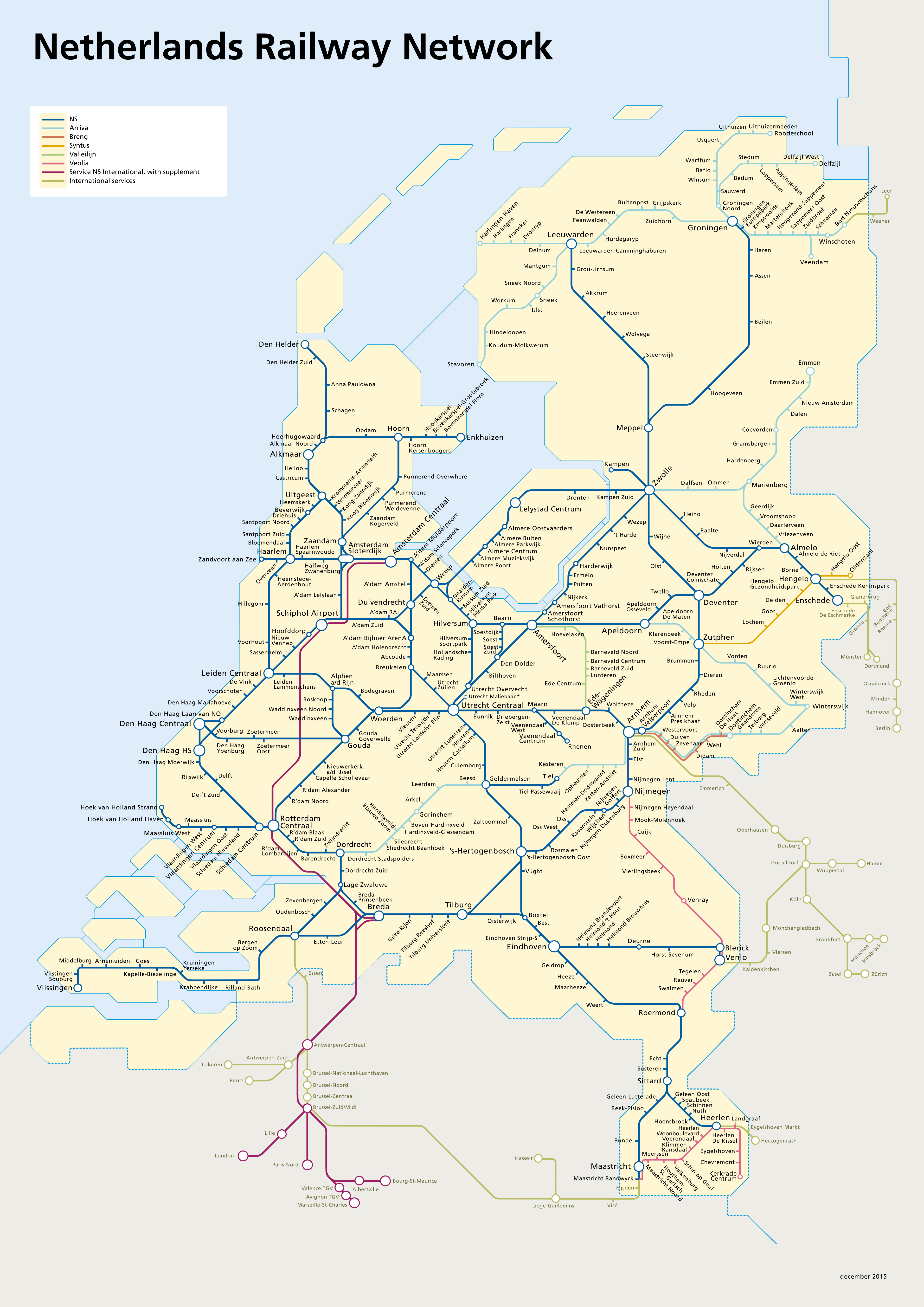
A (slightly outdated) map of the Dutch railway network. — A (slightly) outdated map of the Dutch railway network. Click on the image for a larger version. Reproduced without permission, because I found the original a bit hard to read.

A public transport network map is technically a graph, with nodes and edges. In our case, nodes are train stations, while edges represent trips that can be made between two nodes without leaving the train. Normal people would use a graph databases like Neo4j to store such a graph, but I’m not a normal person so we’ll need to find a way to store this graph in a relational database (side note: I actually already did this in an earlier article.).

node

For simplicity’s sake we’re going to combine stops that are very similar to each other. For instance, instead of the 13 “Nijmegen” stops that we saw earlier, we now only need one node that represents the entire station, including all of its platforms.

We’ll also add a node_id field to the stop table, so that we can keep track of the relationship between nodes in the graph and corresponding stops in the timetable.

id	name
21678	Amsterdam Amstel
21679	Amsterdam Bijlmer ArenA
21680	Amsterdam Centraal
21473	Amsterdam Science Park
21392	Nijmegen
21598	Nijmegen Dukenburg
21601	Nijmegen Heyendaal

edge

Edges can be created from stop_time by joining the table with itself in such a way that the result contains every way to travel directly from one node to another.

Of course, not all edges are equal, so we also need to assign weights to each edge. I haven’t really thought this part through, so I’m just going to use the traversed distance (along the route) and the total number of stops that will be made by the train.

Sometimes there are multiple ways to travel between nodes, e.g. two nodes might be directly connected by an intercity (express) service, or a local train that takes a meandering route. In such cases we’ll store the shortest distance and number of stops as the weights.

id	from_node_id	to_node_id	distance	stops
7782	21680	21392	114717	6
7811	21680	21473	4917	2
7877	21680	21678	5920	2
7878	21680	21679	10256	4

The resulting graph for the Dutch train network contains 479 nodes (side note: The actual number of nodes is 22,152, but most are only served by buses, trams, metros and ferries, and are thus disconnected from the graph.) and 10,655 edges.

Poor man’s pathfinding

Now that we have a graph with weighted edges, we can start working on a pathfinding algorithm. SQL isn’t exactly known as a nice programming language, so to make my life easier I’m not going to use a fancy solution like scalable transfer patterns, but an approach that resembles the horrendously inefficient – but easy to implement – breadth-first search (BFS) algorithm.

BFS is an algorithm that can find the shortest path between a start node and a destination node in a graph. It does this by iteratively exploring the graph “layer by layer”, where each layer consists of nodes that are directly adjacent to the current node and have not been visited yet. This process is repeated until the algorithm has found a path to the destination node or has traversed the entire graph.

I expect that our implementation will be very unoptimised and slow. To ease the pain somewhat I’ll try to limit our search to only a part of the graph. The following query determines which nodes can be visited by our pathfinding algorithm:

SELECT DISTINCT
    node_id
FROM
    stop
INNER JOIN (
    SELECT
        -- 0.25 latitude and 0.20 longitude should be roughly equivalent
        -- to 22 kilometres in the Netherlands
        MIN(latitude)  - 0.25 AS min_lat,
        MAX(latitude)  + 0.25 AS max_lat,
        MIN(longitude) - 0.20 AS min_lon,
        MAX(longitude) + 0.20 AS max_lon
    FROM
        stop
    WHERE
        node_id IN (
            21601, -- Nijmegen Heyendaal (start)
            21473  -- Amsterdam Science Park (destination)
        )
) bounding_box ON
    latitude BETWEEN min_lat AND max_lat
    AND
    longitude BETWEEN min_lon AND max_lon
    AND
    -- This is a stupid hack to remove anything that’s not clearly a
    -- train station, as bus/tram/metro stops in this dataset tend to
    -- have names that include both a place and a street name, e.g.
    -- “Amsterdam, Rokin”.
    name NOT LIKE '%,%'

The query above first computes a rectangular bounding box that encompasses the start (21601) and destination node (21473), and adds a margin (side note: Or is it padding?) of roughly 22 kilometres to its edges to allow for “L-shaped” paths through the graph; it then determines which nodes are located within this bounding box.

Common table expressions

We’ll implement our pathfinding algorithm using common table expressions. A common table expression (CTE) is a named temporary result set that can be used as a reusable building block within the scope of a single SQL statement, almost as if it were a view.

Although this may sound a bit vague, it’s actually quite simple. In the snippet below we convert our previous query into a CTE named allowed_node, and use it to find all of Nijmegen’s train stations that are located within our search space:

WITH allowed_node (node_id) AS (
    SELECT DISTINCT
        node_id
    FROM
        stop
    INNER JOIN (
        SELECT
            -- 0.25 latitude and 0.20 longitude should be roughly equivalent
            -- to 22 kilometres in the Netherlands
            MIN(latitude)  - 0.25 AS min_lat,
            MAX(latitude)  + 0.25 AS max_lat,
            MIN(longitude) - 0.25 AS min_lon,
            MAX(longitude) + 0.25 AS max_lon
        FROM
            stop
        WHERE
            node_id IN (
                21601, -- Nijmegen Heyendaal (start)
                21473  -- Amsterdam Science Park (destination)
            )
    ) bounding_box ON
        latitude BETWEEN min_lat AND max_lat
        AND
        longitude BETWEEN min_lon AND max_lon
        AND
        -- This is a stupid hack to remove anything that’s not clearly a
        -- train station, as bus/tram/metro stops in this dataset tend to
        -- have names that include both a place and a street name, e.g.
        -- “Amsterdam, Rokin”.
        name NOT LIKE '%,%'
)
SELECT
    *
FROM
    node
WHERE
    id IN (SELECT node_id FROM allowed_node)
    AND
    name LIKE 'Nijmegen%'
ORDER BY
    1

As you can see, it’s just like querying a normal table – except that now we define that table within the same query and the CTE ceases to exist once the query has finished.

According to this query, the city of Nijmegen has five train stations that may be considered by our pathfinding algorithm for journeys between Nijmegen Heyendaal and Amsterdam Science Park:

id	name
21392	Nijmegen
21598	Nijmegen Dukenburg
21601	Nijmegen Heyendaal
21603	Nijmegen Lent
21803	Nijmegen Goffert

Finding adjacent nodes

As I mentioned earlier, the first step of our pathfinding algorithm involves finding nodes that are directly adjacent to the start node. The code snippet below shows that we can easily do this by querying the edge table. Feel free to ignore the non-highlighted parts; they’re still the same as in the previous snippet.

WITH allowed_node (node_id) AS (
    SELECT DISTINCT
        node_id
    FROM
        stop
    INNER JOIN (
        SELECT
            -- 0.25 latitude and 0.20 longitude should be roughly equivalent
            -- to 22 kilometres in the Netherlands
            MIN(latitude)  - 0.25 AS min_lat,
            MAX(latitude)  + 0.25 AS max_lat,
            MIN(longitude) - 0.25 AS min_lon,
            MAX(longitude) + 0.25 AS max_lon
        FROM
            stop
        WHERE
            node_id IN (
                21601, -- Nijmegen Heyendaal (start)
                21473  -- Amsterdam Science Park (destination)
            )
    ) bounding_box ON
        latitude BETWEEN min_lat AND max_lat
        AND
        longitude BETWEEN min_lon AND max_lon
        AND
        -- This is a stupid hack to remove anything that’s not clearly a
        -- train station, as bus/tram/metro stops in this dataset tend to
        -- have names that include both a place and a street name, e.g.
        -- “Amsterdam, Rokin”.
        name NOT LIKE '%,%'
)
SELECT
    CONCAT(from_node_id, ' – ', to_node_id) AS path,
    stops,
    distance
FROM
    edge
WHERE
    from_node_id = 21601 -- Nijmegen Heyendaal (start)
    AND
    to_node_id IN (SELECT node_id FROM allowed_node)
ORDER BY
    stops,
    distance

Executing this query gives us the following result:

path	stops	distance
21601 – 21392	1	2295
21601 – 21800	1	7225
21601 – 21761	2	11984
21601 – 21554	3	22167
21601 – 21746	4	29271

There are five stations that can be reached directly (side note: i.e. without a transfer) from Nijmegen Heyendaal and are located within the bounding box that we defined in our allowed_node CTE: 21392 (Nijmegen), 21800 (Mook-Molenhoek), 21761 (Cuijk), 21544 (Boxmeer), and 21746 (Vierlingsbeek).

Let’s make it recursive

We could execute a second (and possibly a third, a fourth, a fifth…) query just like the one above until we find our destination node. But we don‘t have to! Common table expressions can be recursive, which means it’s technically possible to do this ad infinitum (side note: Actually, our algorithm is so slow that it might as well have an infinite execution time. 🤡).

A recursive (and very chonky) version of the previous query can be found below. Again, feel free to ignore the parts that haven’t been highlighted.

WITH RECURSIVE
    allowed_node (node_id) AS (
        SELECT DISTINCT
            node_id
        FROM
            stop
        INNER JOIN (
            SELECT
                -- 0.25 latitude and 0.20 longitude should be roughly equivalent
                -- to 22 kilometres in the Netherlands
                MIN(latitude)  - 0.25 AS min_lat,
                MAX(latitude)  + 0.25 AS max_lat,
                MIN(longitude) - 0.25 AS min_lon,
                MAX(longitude) + 0.25 AS max_lon
            FROM
                stop
            WHERE
                node_id IN (
                    21601, -- Nijmegen Heyendaal (start)
                    21473  -- Amsterdam Science Park (destination)
                )
        ) bounding_box ON
            latitude BETWEEN min_lat AND max_lat
            AND
            longitude BETWEEN min_lon AND max_lon
            AND
            -- This is a stupid hack to remove anything that’s not clearly a
            -- train station, as bus/tram/metro stops in this dataset tend to
            -- have names that include both a place and a street name, e.g.
            -- “Amsterdam, Rokin”.
            name NOT LIKE '%,%'
    ),
    possible_path (nodes, transfers, stops, distance, current_node) AS (
        -- Base case
        SELECT
            CONCAT(' – ', CAST(from_node_id AS CHAR(255)), ' – '),
            0,
            stops,
            distance,
            to_node_id
        FROM
            edge
        WHERE
            from_node_id = 21601 -- Nijmegen Heyendaal (start)
            AND
            to_node_id IN (SELECT node_id FROM allowed_node)

        UNION ALL

        -- Recursive case
        SELECT
            CONCAT(nodes, from_node_id, ' – '),
            transfers + 1,
            possible_path.stops + edge.stops,
            possible_path.distance + edge.distance,
            to_node_id
        FROM
            possible_path
        INNER JOIN
            edge ON
                current_node = from_node_id
        WHERE
            -- Only consider nodes within that rectangular bounding box that we
            -- discussed earlier.
            to_node_id IN (SELECT node_id FROM allowed_node)
            AND
            -- Used to detect cycles within a possible path. It makes no sense
            -- to visit the same station twice!
            nodes NOT LIKE CONCAT('% – ', to_node_id, ' – %')
            AND
            -- This basically sets the number of “layers” that our pathfinding
            -- algorithm is allowed to explore. With transfers set to 3, the
            -- execution time is roughly a second on my machine. With 4 it’s
            -- about 20 seconds. I haven’t tried to set it to 5, but it’ll
            -- probably take *very* long to complete.
            transfers < 3
    )
SELECT DISTINCT
    -- The SUBSTRING() is used to remove the leading “ – ” that we added in the
    -- base case.
    SUBSTRING(CONCAT(nodes, current_node), 4) AS path,
    transfers,
    stops,
    distance
FROM
    possible_path
WHERE
    current_node = 21473 -- Amsterdam Science Park (destination)
ORDER BY
    -- This seems to work reasonably well as a way to score different paths. The
    -- basic idea is that direct connections (fewer transfers) are preferred
    -- over journeys with many transfers, and intercity/express trains (fewer
    -- stops) are preferred over slower, local trains (many stops).
    transfers * stops,
    distance
LIMIT
    5 -- Completely arbitrary limit

There’s a lot to unpack here, so let’s break it down.

We added the RECURSIVE keyword on the first line to indicate that at least one of the common table expressions in this statement is recursive.

The allowed_node CTE hasn’t changed, but we have added a second possible_path CTE that works recursively. This CTE has five fields (nodes, transfers, stops, distance and current_node) and consists of two parts: a base case and a recursive case, which are combined into a single result set using some UNION ALL magic.

The base case handles the first leg of the journey. It’s a modified version of the previous query. We have added two new fields, transfers and current_node. transfers keeps track of the number of times that a traveller would have to change trains, while current_node is the id of the node that is being visited by the pathfinding algorithm.

The recursive case handles all parts of the journey that require a transfer. This is where most of the magic happens. The base case previously yielded a set of all nodes that can be reached directly from the start node. In the recursive case, we now do the same for each of those adjacent nodes. Having said that, it differs from the base case in several ways:

We now need to keep track of state. This is done in three ways: The sequence of visited nodes is stored as a string, to which we append new nodes using the CONCAT() function. The number of transfers and stops, and travelled distance are stored as integers and modified using addition (+). Finally, the to_node_id from the previous case is simply overwritten with the new value.
To make sure we don’t visit a station more than once, we verify that a node isn’t already part of a sequence of nodes.
It’d also be nice if the recursion terminates at some point. The query above achieves this by limiting the maximum number of transfers to 3. This doesn’t make a lot of sense for a real journey planner, but is good enough for our little toy project.

Querying the recursive possible_path CTE is easy. We simply select from possible_path as if it were a regular table. The destination node can be set using the WHERE clause.

You might be wondering why we don’t also filter by the start node here. That’s because it’s still hardcoded inside the possible_path CTE. This is done for stupid performance reasons; it appears that MySQL struggles to cache intermediate query results when we convert it into a variable. It’s ugly, but it gets the job done.

Anyway, executing this query gives us the following result:

path	transfers	stops	distance
21601 – 21392 – 21680 – 21473	2	9	121928
21601 – 21392 – 21671 – 21473	2	11	131837
21601 – 21392 – 21678 – 21618 – 21473	3	8	114842
21601 – 21392 – 21251 – 21473	2	13	143748
21601 – 21392 – 21680 – 21618 – 21473	3	9	121927

Here is a slightly different version of that same table that uses node names in place of meaningless ids:

path	transfers	stops	distance
Nijmegen Heyendaal – Nijmegen – Amsterdam Centraal – Amsterdam Science Park	2	9	121928
Nijmegen Heyendaal – Nijmegen – Amsterdam Sloterdijk – Amsterdam Science Park	2	11	131837
Nijmegen Heyendaal – Nijmegen – Amsterdam Amstel – Amsterdam Muiderpoort – Amsterdam Science Park	3	8	114842
Nijmegen Heyendaal – Nijmegen – Schiphol Airport – Amsterdam Science Park	2	13	143748
Nijmegen Heyendaal – Nijmegen – Amsterdam Centraal – Amsterdam Muiderpoort – Amsterdam Science Park	3	9	121927

As it turns out, the path in the first row is indeed the best way to travel from Nijmegen Heyendaal to Amsterdam Science Park!

We can’t pat ourselves on the back yet though, because this still doesn’t tell us which trains we should take. Head over to part 2 if you’re eager to find out how that works!